Essential Dynamics Analysis
Synopsis
This example shows how to perform essential dynamics analysis of molecular
dynamics (MD) trajectories. A EDA instance that stores covariance
matrix and principal modes that describes the essential dynamics of the system
observed in the simulation will be built. EDA and principal modes
(Mode) can be used as input to functions in dynamics module
for further analysis.
User needs to provide trajectory in DCD file format and PDB file of the system.
Example input:
Setup environment
We start by importing everything from ProDy:
In [1]: from prody import *

In [2]: from pylab import *

In [3]: ion()
Parse reference structure
The PDB file provided with this example contains and X-ray structure which will be useful in a number of places, so let’s start with parsing this file first:
In [4]: structure = parsePDB('mdm2.pdb')

In [5]: structure
Out[5]: <AtomGroup: mdm2 (1449 atoms)>
This function returned a AtomGroup instance that
stores all atomic data parsed from the PDB file.
EDA calculations
Essential dynamics analysis (EDA or PCA) of a trajectory can be performed in two ways.
Small files
If you are analyzing a small trajectory, you can use an Ensemble
instance obtained by parsing the trajectory at once using parseDCD():
In [6]: ensemble = parseDCD('mdm2.dcd')

In [7]: ensemble.setCoords(structure)

In [8]: ensemble.setAtoms(structure.calpha)

In [9]: ensemble
Out[9]: <Ensemble: mdm2 (0:500:1) (500 conformations; selected 85 of 1449 atoms)>

In [10]: ensemble.superpose()

In [11]: eda_ensemble = EDA('MDM2 Ensemble')

In [12]: eda_ensemble.buildCovariance( ensemble )

In [13]: eda_ensemble.calcModes()

In [14]: eda_ensemble
Out[14]: <EDA: MDM2 Ensemble (20 modes; 85 atoms)>
Large files
If you are analyzing a large trajectory, you can pass the trajectory instance
to the PCA.buildCovariance() method as follows:
In [15]: dcd = DCDFile('mdm2.dcd')

In [16]: dcd.link(structure)

In [17]: dcd.setAtoms(structure.calpha)

In [18]: dcd
Out[18]: <DCDFile: mdm2 (linked to AtomGroup mdm2; next 0 of 500 frames; selected 85 of 1449 atoms)>

In [19]: eda_trajectory = EDA('MDM2 Trajectory')

In [20]: eda_trajectory.buildCovariance( dcd )

In [21]: eda_trajectory.calcModes()

In [22]: eda_trajectory
Out[22]: <EDA: MDM2 Trajectory (20 modes; 85 atoms)>
Comparison
In [23]: printOverlapTable(eda_ensemble[:3], eda_trajectory[:3])
Overlap Table
                       EDA MDM2 Trajectory
                         #1     #2     #3
EDA MDM2 Ensemble #1   +1.00   0.00   0.00
EDA MDM2 Ensemble #2    0.00  +1.00   0.00
EDA MDM2 Ensemble #3    0.00   0.00  +1.00
Overlap values of +1 along the diagonal of the table shows that top ranking 3 essential (principal) modes are the same.
Multiple files
It is also possible to analyze multiple trajectory files without concatenating them. In this case we will use data from two independent simulations
In [24]: trajectory = Trajectory('mdm2.dcd')

In [25]: trajectory.addFile('mdm2sim2.dcd')

In [26]: trajectory
Out[26]: <Trajectory: mdm2 (2 files; next 0 of 1000 frames; 1449 atoms)>

In [27]: trajectory.link(structure)

In [28]: trajectory.setCoords(structure)

In [29]: trajectory.setAtoms(structure.calpha)

In [30]: trajectory
Out[30]: <Trajectory: mdm2 (linked to AtomGroup mdm2; 2 files; next 0 of 1000 frames; selected 85 of 1449 atoms)>

In [31]: eda = EDA('mdm2')

In [32]: eda.buildCovariance( trajectory )

In [33]: eda.calcModes()

In [34]: eda
Out[34]: <EDA: mdm2 (20 modes; 85 atoms)>
Save your work
You can save your work using ProDy function saveModel(). This will
allow you to avoid repeating calculations when you return to your work later:
In [35]: saveModel(eda)
Out[35]: 'mdm2.eda.npz'
loadModel() function can be used to load this object without any loss.
Analysis
Let’s print fraction of variance for top raking 4 essential modes:
In [36]: for mode in eda_trajectory[:4]:
   ....:     print(calcFractVariance(mode).round(2))
   ....:
0.26
0.11
0.08
0.06
You can find more analysis functions in Dynamics Analysis.
Plotting
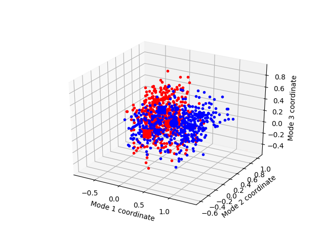
Now, let’s project the trajectories onto top three essential modes:
In [37]: mdm2ca_sim1 = trajectory[:500]

In [38]: mdm2ca_sim1.superpose()

In [39]: mdm2ca_sim2 = trajectory[500:]

In [40]: mdm2ca_sim2.superpose()

# We project independent trajectories in different color
In [41]: showProjection(mdm2ca_sim1, eda[:3], color='red', marker='.');

In [42]: showProjection(mdm2ca_sim2, eda[:3], color='blue', marker='.');

# Now let's mark the beginning of the trajectory with a circle
In [43]: showProjection(mdm2ca_sim1[0], eda[:3], color='red', marker='o', ms=12);

In [44]: showProjection(mdm2ca_sim2[0], eda[:3], color='blue', marker='o', ms=12);

# Now let's mark the end of the trajectory with a square
In [45]: showProjection(mdm2ca_sim1[-1], eda[:3], color='red', marker='s', ms=12);

In [46]: showProjection(mdm2ca_sim2[-1], eda[:3], color='blue', marker='s', ms=12);
You can find more plotting functions in Dynamics Analysis and Measurement Tools modules.
Visualization
The above projection is shown for illustration. Interpreting the essential modes and projection of snapshots onto them is case dependent. One should know what kind of motion the top essential modes describe. You can use Normal Mode Wizard for visualizing essential mode shapes and fluctuations along these modes.
We can write essential modes in NMD Format for NMWiz as follows:
In [47]: writeNMD('mdm2_eda.nmd', eda[:3], structure.select('calpha'))
Out[47]: 'mdm2_eda.nmd'