Core Calculations
In order to infer signature dynamics features we create mode ensembles from the
PDB ensembles by calculating normal modes for each member of the
PDBEnsemble as in the previous page or [SZ18].
First, make necessary imports from ProDy and Matplotlib packages if you haven’t already.
In [1]: from prody import *

In [2]: from pylab import *

In [3]: ion()
Mode Ensemble
For this analysis we’ll use the PDBEnsemble object,
which we just created, to build a ModeEnsemble.
There are options to select the model (GNM by default) and the way of
considering non-aligned residues (default is reduceModel(), which treats
them as environment).
If necessary, we first load the ensemble:
In [4]: ens = loadEnsemble('LeuT.ens.npz')
Then we calculated first 20 GNM modes for each member of the ensemble:
In [5]: gnms = calcEnsembleENMs(ens, model=GNM, trim='reduce', n_modes=20, match=True)

In [6]: gnms
Out[6]: <ModeEnsemble: 103 modesets (20 modes, 510 atoms)>
In this way, we will obtain one ModeSet for each member and 85 in total.
Finding a consistent order of modes across different mode sets is critical to the
accuracy of SignDy calculations. Therefore, in the above code, match is set
to True so that all other ModeSet`s are sorted to match the order of
the reference :class:.ModeSet`, which is the first ModeSet in the
ModeEnsemble by default.
Signature Dynamics
Signature dynamics are calculated as the mean and standard deviation of various properties such as mode shapes and mean square fluctations.
For example, we can show the average and standard deviation of the shape of the first mode (second index 0). The first index of the mode ensemble is over conformations.
In [7]: showSignatureMode(gnms[:, 0]);
In the plot, the curve shows the mean values, the darker shade shows the standard deviations, and the lighter shade shows the range (minimum and maximum values). We can also show such things for properties involving multiple modes such as the mean square fluctuations from the first 5 modes,
In [8]: showSignatureSqFlucts(gnms[:, :5]);
or the cross-correlations from the first 20.
In [9]: showSignatureCrossCorr(gnms[:, :20]);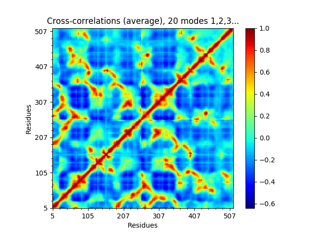
We can also look at distributions over values across different members of the ensemble such as inverse eigenvalue. We can show a bar above this with individual members labelled like [JK15].
In [10]: highlights = {'2A65A': 'LeuT:OF', '3TT3A': 'LeuT:IF'}

In [11]: from matplotlib.gridspec import GridSpec

In [12]: gs = GridSpec(ncols=1, nrows=2, height_ratios=[1, 10], hspace=0.15)

In [13]: subplot(gs[0]);

In [14]: showVarianceBar(gnms[:, :5], fraction=True, highlights=highlights);

In [15]: xlabel('');

In [16]: subplot(gs[1]);

In [17]: showSignatureVariances(gnms[:, :5], fraction=True, bins=80, alpha=0.7);

In [18]: xlabel('Mode weight');

Saving the ModeEnsemble
Finally we save the mode ensemble for later processing:
In [19]: saveModeEnsemble(gnms, 'LeuT')
Out[19]: 'LeuT.modeens.npz'