Evolution Analysis
This part follows from MSA Files. The aim of this part is to show how to calculate residue conservation and coevolution properties based on multiple sequence alignments (MSAs). MSA
First, we import everything from the ProDy package.
In [1]: from prody import *

In [2]: from pylab import *

In [3]: ion()  # turn interactive mode on
Get MSA data
Let’s download full MSA file for protein family RnaseA. We can do this by specifying the PDB ID of a protein in this family.
In [4]: searchPfam('1K2A').keys()
Out[4]: ['PF00074']
In [5]: fetchPfamMSA('PF00074')
Out[5]: 'PF00074_full.sth'
Let’s parse the downloaded file:
In [6]: msa = parseMSA('PF00074_full.sth')
Refine MSA
Here, we refine the MSA to decrease the number of gaps. We will remove any
columns in the alignment for which there is a gap in the specified PDB file,
and then remove any rows that have more than 20% gaps. refineMSA()
does all of this and returns an MSA object.
In [7]: msa_refine = refineMSA(msa, label='RNAS2_HUMAN', rowocc=0.8, seqid=0.98)

In [8]: msa_refine
Out[8]: <MSA: PF00074_full refined (label=RNAS2_HUMAN, rowocc>=0.8, seqid>=0.98) (698 sequences, 126 residues)>
MSA is refined based on the sequence of RNAS2_HUMAN, corresponding to 1K2A.
Occupancy calculation
Evol plotting functions are prefixed with show. We can plot the occupancy
for each column to see if there are any positions in the MSA that have a lot of
gaps. We use the function showMSAOccupancy() that uses
calcMSAOccupancy() to calculate occupancy for MSA.
In [9]: showMSAOccupancy(msa_refine, occ='res');

Let’s find the minimum:
In [10]: calcMSAOccupancy(msa_refine, occ='res').min()
Out[10]: 0.011461318051575931
We can also specify indices based on the PDB.
In [11]: indices = list(range(5,131))

In [12]: showMSAOccupancy(msa_refine, occ='res', indices=indices);
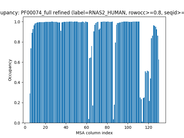
Further refining the MSA to remove positions that have low occupancy will change the start and end positions of the labels in the MSA. This is not corrected automatically on refinement. We can also plot occupancy based on rows for the sequences in the MSA.
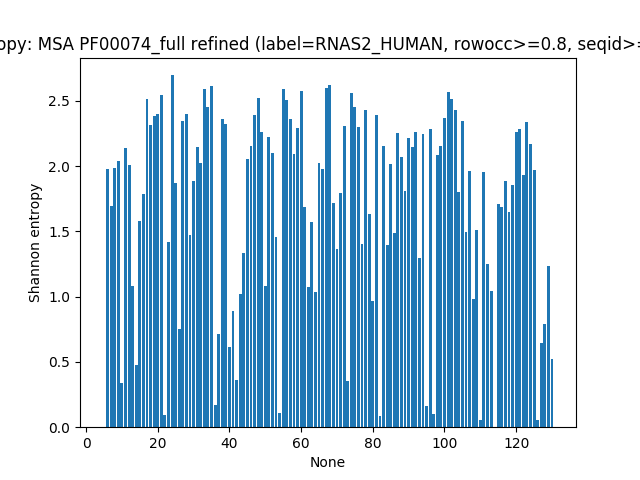
Entropy Calculation
Here, we show how to calculate and plot Shannon Entropy. Entropy for
each position in the MSA is calculated using calcShannonEntropy(). It
takes MSA object or a numpy 2D array containg MSA as input and returns
a 1D numpy array.
In [13]: entropy = calcShannonEntropy(msa_refine)

In [14]: entropy
Out[14]:
array([-0.        ,  1.97536341,  1.6976014 ,  1.98686002,  2.04097927,
        0.33881322,  2.13977922,  2.00661895,  1.08055377,  0.47729866,
        1.58125405,  1.78890686,  2.51747686,  2.31397501,  2.38803313,
        2.40126663,  2.54295735,  0.09338611,  1.41579988,  2.69688922,
        1.8686074 ,  0.75606438,  2.34383631,  2.39720547,  1.47431149,
        1.88334663,  2.14950549,  2.02528004,  2.58853012,  2.45108208,
        2.61723915,  0.16813412,  0.71292546,  2.36093797,  2.32632049,
        0.61799546,  0.89021762,  0.36043225,  1.01850997,  1.33382837,
        2.05607945,  2.15459689,  2.3895889 ,  2.52272713,  2.26277362,
        1.07883485,  2.22209291,  2.10332436,  1.46075956,  0.10580037,
        2.5880002 ,  2.50810725,  2.35814643,  2.09300504,  2.29386782,
        2.5724491 ,  1.68877804,  1.07047455,  1.57433048,  1.03752672,
        2.0206458 ,  1.97820357,  2.60225   ,  2.62010838,  1.71632538,
        1.36403271,  1.79131851,  2.30781167,  0.35730727,  2.55844119,
        2.45589515,  2.30325997,  1.40702068,  2.42986786,  1.63284318,
        0.96868799,  2.39301813,  0.08317819,  2.15806993,  1.39390954,
        2.01888973,  1.48477641,  2.25039015,  2.071024  ,  1.80876533,
        2.21861345,  2.1495278 ,  2.26531537,  1.29842729,  2.2432391 ,
        0.16590041,  2.28183392,  0.10492724,  2.08455959,  2.15120138,
        2.36710596,  2.56442544,  2.51541107,  2.42719479,  1.80265513,
        2.34569871,  1.4964265 ,  1.96057778,  0.98329793,  1.51199785,
        0.05404462,  1.95389007,  1.24837514,  1.04713865, -0.        ,
        1.71085363,  1.68585224,  1.88812929,  1.64865814,  1.8563798 ,
        2.26222015,  2.28490399,  1.93257978,  2.34153018,  2.17263465,
        1.97322381,  0.05898735,  0.64841109,  0.79058895,  1.23695064,
        0.52622679])
entropy is a 1D NumPy array. Plotting is done using
showShannonEntropy().
In [15]: showShannonEntropy(msa_refine, indices);
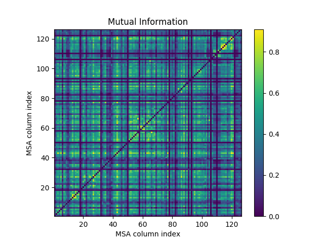
Mutual Information
We can calculate mutual information between the positions of the MSA using
buildMutinfoMatrix() which also takes an MSA object
or a numpy 2D array containing MSA as input.
In [16]: mutinfo = buildMutinfoMatrix(msa_refine)

In [17]: mutinfo
Out[17]:
array([[0.        , 0.20631824, 0.16401097, ..., 0.06095202, 0.14566864,
        0.05380968],
       [0.20631824, 0.        , 0.60253758, ..., 0.22563382, 0.22440521,
        0.18667669],
       [0.16401097, 0.60253758, 0.        , ..., 0.35108633, 0.37773013,
        0.24761374],
       ...,
       [0.06095202, 0.22563382, 0.35108633, ..., 0.        , 0.4087536 ,
        0.22060682],
       [0.14566864, 0.22440521, 0.37773013, ..., 0.4087536 , 0.        ,
        0.27725374],
       [0.05380968, 0.18667669, 0.24761374, ..., 0.22060682, 0.27725374,
        0.        ]])
Result is a 2D NumPy array.
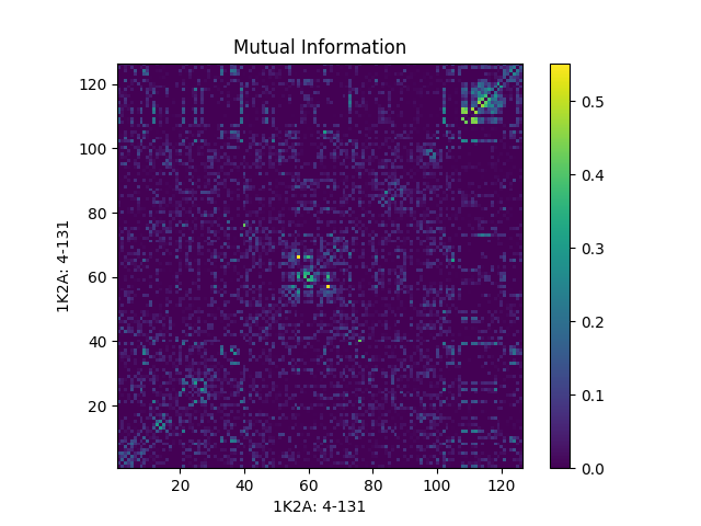
We can also apply normalization using applyMutinfoNorm() and
correction using applyMutinfoCorr() to the mutual information matrix
based on references [Martin05] and [Dunn08], respectively.
| [Martin05] | Martin LC, Gloor GB, Dunn SD, Wahl LM. Using information theory to search for co-evolving residues in proteins. Bioinformatics 2005 21(22):4116-4124. |
| [Dunn08] | Dunn SD, Wahl LM, Gloor GB. Mutual information without the influence of phylogeny or entropy dramatically improves residue contact prediction. Bioinformatics 2008 24(3):333-340. |
In [18]: mutinfo_norm = applyMutinfoNorm(mutinfo, entropy, norm='minent')

In [19]: mutinfo_corr = applyMutinfoCorr(mutinfo, corr='apc')
Note that by default norm="sument" normalization is applied in
applyMutinfoNorm and corr="prod" is applied in applyMutinfoCorr.
Now we plot the mutual information matrices that we obtained above and see the effects of different corrections and normalizations.
In [20]: showMutinfoMatrix(mutinfo);
In [21]: showMutinfoMatrix(mutinfo_corr, clim=[0, mutinfo_corr.max()],
   ....:    xlabel='1K2A: 4-131');
   ....:
Output Results
Here we show how to write the mutual information and entropy arrays to file.
We use the writeArray() to write NumPy array data.
In [22]: writeArray('1K2A_MI.txt', mutinfo)
Out[22]: '1K2A_MI.txt'
This can be later loaded using parseArray().
Rank-ordering
Further analysis can also be done by rank ordering the matrix and analyzing
the pairs with highest mutual information or the most co-evolving residues.
This is done using calcRankorder(). A z-score normalization can also
be applied to select coevolving pairs based on a z score cutoff.
In [23]: rank_row, rank_col, zscore_sort = calcRankorder(mutinfo, zscore=True)

In [24]: asarray(indices)[rank_row[:5]]
Out[24]: array([127,  31,  31, 128, 115])

In [25]: asarray(indices)[rank_col[:5]]
Out[25]: array([126,  26,  29, 126, 113])

In [26]: zscore_sort[:5]
Out[26]: array([4.50792926, 3.55425262, 3.42345689, 3.27298657, 3.21999586])